Profiling¶

Introduction¶

Profiling is the process and tools used for performance analysis of an application or piece of software. This involves executing the application while instrumented with performance probes (timing and counters) so that one can determine where the time is spent and focus on bottlenecks ("hotspots"). There are typically 2 modes: sampling mode and tracing mode. Sampling is less intrusive because it tries to limit its capture to just some representative results. Tracing mode is very intrusive, because it gives exact counts and timing. Sampling mode can give you an idea of what is going on but often the details are fuzzy/inexact. Tracing mode gives you the full picture but the application runs very slowly. The results are relatively correct but the time amounts are much longer than when there is no tracing.

Although VisualVM is included in the JDKs up to Java 8, it is not very useful for tracing mode profiling. We have found that in real applications, sometimes VisualVM will just freeze itself and the application. CPU sampling mode works OK and is useful for finding high-level hot spots, though it can be misleading at times. Information on VisualVM included in the JDK can be found at https://docs.oracle.com/javase/8/docs/technotes/guides/visualvm/.

In our experience, the commercial product Yourkit is significantly better for profiling. It requires running the target JVM with an agent. The absolute times are greatly inflated because of the profiling overhead, but the call counts and relative times seem quite accurate.

VisualVM can be useful for enabling and capturing the output of specific JMX MBean instrumentation that has been placed in the FWD code. These locations can be very useful for targeted measurement of performance and timing. See the

How to Enable Tracing¶

TBD

Analysis Tips¶

Merged Callees¶

This section is specific to Yourkit.

A very useful view is the Merged Callees tree, where you can manually expand the nodes that are time consuming. This is taken from a CPU profiling snapshot, captured in tracing mode (not async sampling mode). This is the slowest mode, but it's not too bad when you are tracing a well-defined, relatively short operation, like opening a single screen.

After capturing and opening the snapshot, open either the Hot spots or the Method list views, select a method in the top part of the screen, then select the Merged Callees view in the bottom part of the screen. From there, you can open/close individual nodes in the tree.

How to Find a Problematic Method¶

Sometimes a problematic method may be difficult to find. For example, it may not appear in a list of hotspots but it could still be a significant bottleneck (in Yourkit, items in Method list which are not mentioned in the Hot spots window).

One can look for methods which consume higher than some threshold of the overall, aggregate time. Initial analysis will use a threshold somewhere between 5-10%, which generally will appear as a hotspot (in Yourkit they will appear in the Hot spots view). As fixes are incorporated, the most obvious items will be removed. This makes the bottlenecks less obvious to find. Thar means the threshold will be reduced and at that point one might look for methods that are at least 1-3% of the overall aggregate time.

Bottlenecks in FWD¶

When profiling FWD itself, one will usually ignore the runtime methods whose main purpose it is to invoke converted business logic, like the ControlFlowOps.invoke*() methods or the BlockManager workers. Those methods are hard to navigate, because the call tree from those points downward is very deep.

Focus on methods which actually result in work which takes a long time in the FWD runtime itself, or in third party code called from FWD (e.g. H2).

In Yourkit, there is also SQL information ("Events -> Events by Table"), to find slow queries, to see if there is something wrong with the way the query is formed. YourKit records the SQL that was executed, but unfortunately not the substitution parameters that were passed.

Bottlenecks in Converted Code¶

The same techniques described above can be used with the converted code (which is just Java after all). The key difference is that one may want to exclude the FWD runtime classes from the analysis so that it does not obscure the application code bottlenecks. The FWD runtime will be involved with everything being processed in the converted code. If it is not excluded then the hotspots may appear to be in FWD instead of the application.

TBD: add more details here.

JMX MBean Instrumentation¶

Introduction¶

For an introduction to MBeans see https://www.baeldung.com/java-management-extensions

The JMX MBean infrastructure and some instrumentation was added to FWD v4 starting in task branch 3821c revision 11645 (see #4785-746 and the following notes). It will be further enhanced in #1849.

Design¶

There are several types of counters defined in the com.goldencode.p2j.jmx package.

SimpleLongCounter - contains two long fields. The update operation accepts a long argument. The value of the argument is added to the total field. The count field is incremented by 1.
SimpleMapCounter - holds a map of named SimpleLongCounter counters. An update operation provides a name of the counter and a long update for it.
NanoCounter - a counter for measuring execution times. Contains the same fields as SimpleLongCounter but contains a timer method which accepts an Operation (a Functional interface that is a 'Runnable that can throw Exception'). The operation is called and the elapsed time is used to update the values of total and count. See the ServerState class for an example.

      NANO_TIMER.timer(() ->  setWidgetAttrs((Object[])PayloadSerializer.readPayload(in)));

Every instance of the counter contains its own enabled flag to minimize the overhead for checking if it is enabled. The MBean propagates the changes of this flag to all its instances on update. See Facultative class implementation for the details. So when all MBeans are disabled the runtime overhead is negligible.

Usage¶

By default all counters are disabled. To enable you can use VisualVM with the VisualVM-MBeans plugin. It is also possible to use JConsole but it is more effort. These instructions will demonstrate usage with VisualVM.

You have to install the VisualVM-MBeans plugin. Open Tools->Plusins menu and add VisialVM-MBeans plugin if it is not yet installed: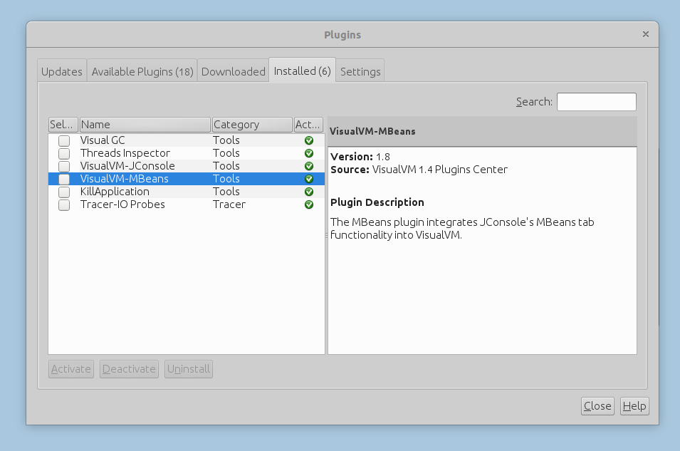

Steps:

1. Connect to a process.

Start VisualVM, select the process, and double click on it. See the screenshot below

2. Switch to the MBeans tab.

FWD MBeans are under com.goldencode.p2j.. For a specific counter, you can see values in the Attributes tab.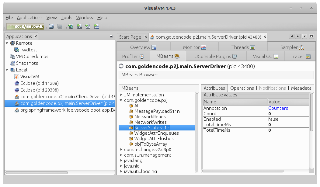

3. Enable/Disable/Reset/Print Counters

In the Operations tab, you can enable/disable/reset the counter. In this tab, you can also print value(s) to a specified file. If the file already exists, the new data will be appended. The value of the Annotation attribute will be included in the output.

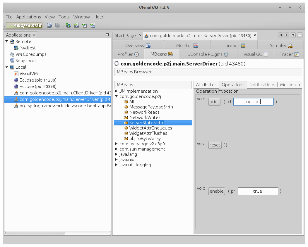
The All section allows one to change annotation and enable/disable/reset/print all defined counters in one operation.

Adding Tracepoints¶

To add a new instrumentation location, just add a new member to the corresponding enum in the FwdJMX class and modify the application code to use it.

For example, imagine that we want to measure how much CPU time takes the decryption of the SSL traffic. More specifically - the total CPU time consumed by the SSL.unwrap() method which is called in the SSL.doUnwrap() method:

         unwrapResult = engine.unwrap(outUnwrap, inpUnwrap);

We have to do the following:

Add sslUnwrap member to the FwdJMX.TimeStat enum.

      /** ServerStat.widgetAttrs (de)serialization */
      ServerStateS11n,
      /** Message.payload (de)serialization */
      MessagePayloadS11n,
      /** Protocol.objToByteArray */
      objToByteArray,
      /** SSL.doUnwrap */
      sslUnwrap;

Define a static member private static final NanoTimer UNWRAP_TIMER = NanoTimer.getInstance(FwdJMX.TimeStat.sslUnwrap); in the SSL class.

Replace

         unwrapResult = engine.unwrap(outUnwrap, inpUnwrap);

with

         AtomicReference<SSLEngineResult> holder = new AtomicReference<>();
         UNWRAP_TIMER.timer(() -> holder.set(engine.unwrap(outUnwrap, inpUnwrap)));
         unwrapResult = holder.get();

What was described above in this section works for 'general purpose' counters which are supposed to be used in different situaions.However there can be more specific requirements. In this case one can define a special MBean and its implementation and register it using FwdJMX.register call.
See e.g. the instrumentation of the LockTableUpdater using LockTableUpdaterStatMBean and LockTableUpdaterStat.

JMX Instrumentation Types¶

FWD provides JMX instrumentation to measure various parts of the FWD runtime, grouped under the com.goldencode.p2j name. There is a MBean named All, which provides operations to:

dumpAll(String), write all the JMX instrumentation to a file.
resetAll(), to reset all metrics which are not live representation (timers, counters, etc).
enableAll(boolean), to enable or disable all metrics which are not a live representation (timers, counters, etc).

The basic JMX metrics defined by p2j.jmx.FwdJMX class are:

`TimeStat`¶

This is referenced as TIMER in this documentation, with these attributes and operations:

Attributes

Attribute	Type	Description
`Enabled`	boolean	The metric's state - enabled or disabled.
`Count`	long	The number of executions of this metric.
`TotalTimeMs`	long	Total execution time, in milliseconds.
`TotalTimeNs`	long	Total execution time, in nanoseconds.

Operations

Operation	Description
`void print(String)`	Dump this metric to the specified file.
`void reset()`	Reset this metric.
`void enable(boolean)`	Enable or disable this metric.

`Counter`¶

This is referenced as COUNTER in this documentation, with these cases attributes and operations:

Attributes

Attribute	Type	Description
`Enabled`	boolean	The metric's state - enabled or disabled.
`Count`	long	The number of executions of this metric.
`Total`	long	Total aggregated value of this metric.

Operations

Operation	Description
`void print(String)`	Dump this metric to the specified file.
`void reset()`	Reset this metric.
`void enable(boolean)`	Enable or disable this metric.

`MapCounter`¶

This is referenced as MAP in this documentation, with these cases attributes and operations:

Attributes

Attribute	Type	Description
`Enabled`	boolean	The metric's state - enabled or disabled.
`Count`	long	The number of executions of this metric.
`Total`	long	Total aggregated value of this metric.
`Values`	Map<String, Long>	Aggregated value of this metric, by a specific key.

Operations

Operation	Description
`void print(String)`	Dump this metric to the specified file.
`void reset()`	Reset this metric.
`void enable(boolean)`	Enable or disable this metric.

`QueryProfiler`¶

This is referenced as QUERY in this documentation, a custom metric with these attributes and operations:

Attributes

Attribute	Type	Description
`Enabled`	boolean	The metric's state - enabled or disabled.
`QueryCount`	long	The number of executed queries.
`Values`	Map<String, Map<String, Long>>	For each query, its aggregated value for: * ROWS_COUNT, number of returned rows * CACHE_HITS, number of records read from cache. * CACHE_MISSES, number of records read from the table. * HYDRATE_TOTAL_TIME, total time in nanos spent in hydrating a record.

Operations

Operation	Description
`void print(String)`	Dump this metric to the specified file.
`void reset()`	Reset this metric.
`void enable(boolean)`	Enable or disable this metric.

`LockTableUpdaterStat`¶

This is referenced as LOCK in this documentation, a custom metric to track, for each connected database, the access to the meta _lock table.

Attributes

Attribute	Type	Description
`ActiveLocks`	long	Get number of active locks
`DeletesFromVST`	long	Get number of VST records deleted not in batch.
`LockEvents`	long	Get number of processed lock events.
`PersistCalls`	long	Get the number of calls to persist locks to the meta database
`PersistedLocks`	long	Get number of locks in VST.

Operations

Operation	Description
`void flush()`	Persist locks to the meta database.

Available Instrumentation Points¶

FWD Appserver Agent State Instrumentation¶

Appserver Agents are used for appserver requests as well as REST/SOAP/WebHandler processing. Agent state is being tracked using JMX beans with the name having the AppServer_ prefix followed by the appserver name (like AppServer_hotel, for an appserver name hotel).

Each metric allows these int attributes:

MaxAgents, for the number of maximum agents configured for this appserver.
RunningAgents, for the number of agents running at this point (executing tasks or otherwise waiting for work).
AvailableAgents, for the number of agents currently available for executing tasks.

FWD Server - Persistence and ORM Instrumentation¶

Name	Type	API 2	Description
OrmDynParseFind	TIMER	`DynamiQueryHelper.parseFindQuery`	Dynamic FIND query parse.
OrmDynParseQuery	TIMER	`DynamiQueryHelper.parseQuery`	Dynamic query parse.
OrmHydrateRecord	TIMER	`SQLQuery.hydrateRecord`	Record hydration (from a `ResultSet`)
OrmFqlParse	TIMER	`Query.createSqlQuery`	FQL query parse.
OrmTempTableQuery	TIMER	`UnclosablePreparedStatement`	H2 query `execute` method calls.
OrmDynQueryInterpret	TIMER	`RuntimeJastInterpreter.interpret`	Dynamic query interpret.
OrmHqlHelperParse	TIMER	`HQLHelper.obtain`	Helper for an in-memory state of a converted query (static or dynamic).
OrmPreselectQueryAssemble	TIMER	`PreselectQuery.assembleHQL`	Calculate the final FQL for a converted query (static or dynamic).
OrmCreateDynamicTable	TIMER	`TempTableBuilder.tempTablePrepareImpl`	DATASET-HANDLE parameter processing.
OrmCreateDynamicBuffer	TIMER	`TemporaryBuffer.createDynamicBufferForTempTable`	Dynamic buffer definition.
OrmBufferDefineTemp	TIMER	`TemporaryBuffer.define`	temp-table buffer definition.
OrmBufferDefinePerm	TIMER	`RecordBuffer.define`	permanent schema buffer definition.
OrmBufferDelete	TIMER	`BufferImpl.resourceDelete`	record buffer delete.
OrmTableMapperMap	TIMER	`TableMapper.mapTemporaryTable`	API called during temp-table definition.
OrmTempTableParam	TIMER	`TemporaryBuffer.associate`	TABLE parameter processing.
OrmDynamicTableParam	TIMER	`TemporaryBuffer.createDynamicTable`	TABLE-HANDLE parameter processing.
OrmDataSetParam	TIMER	`DataSet.associate`	DATASET parameter processing.
OrmDynamicDataSetParam	TIMER	`DataSet.createDynamicDataSet`	DATASET-HANDLE parameter processing.
OutputTableCopier	TIMER	`OutputTableCopier.finished`	Processing of a OUTPUT TABLE parameter (at end of call).
OutputTableHandleCopier	TIMER	`OutputTableHandleCopier.finished`	Processing of a OUTPUT TABLE-HANDLE parameter (at end of call).
OutputDataSetCopier	TIMER	`OutputDataSetCopier.finished`	Processing of a OUTPUT DATASET parameter (at end of call).
OutputDataSetHandleCopier	TIMER	`OutputDataSetHandleCopier.finished`	Processing of a OUTPUT DATASET-HANDLE parameter (at end of call).
OrmRedo	TIMER	`Savepoint.maybeReapplyNoUndo`	Processing of REDO operations for NO-UNDO tables after a rollback.
OrmNoUndoTrace	TIMER	`Savepoint.noUndo`	Preparing for eventual REDO operations by logging a redo trace.

FWD Server Runtime Instrumentation¶

Name	Type	API 2	Description
ContextLocalGet	TIMER	`ContextLocal.get`	Context-local state.
MessagePayloadS11n	TIMER	`Message.read/writeExternal`	`Message.payload` (de)serialization
objToByteArray	TIMER	`Protocol.objToByteArray`
ServerStateS11n	TIMER	`p2j.ui.ServerState.read/writeExternal`	`ServerState.widgetAttrValues` (de)serialization
sslSend	TIMER	`SSL.send`	SSL send time
sslWrap	TIMER	`SSL.wrap`	SSL wrap time
sslUnwrap	TIMER	`SSL.unwrap`	SSL unwrap time
TMCommit	TIMER	`TransactionManager.processCommit`	Block commit processing.
TMRollback	TIMER	`TransactionManager.processRollback`	Block rollback processing.
TMValidate	TIMER	`TransactionManager.processValidate`	Block validate processing.

FWD OpenClient Runtime Instrumentation¶

Add this code to enable JMX instrumentation in the FWD OpenClient runtime, preferably at the beginning of the main method:

      FwdJMX.init();

All JMX beans are prefixed with Appserver:

Name	Type	API 2	Description
AppserverAddTableMetaData	TIMER	`LegacyJavaAppserver.addTableMetaData`	Time spent when adding a new table to a graph.
ApperverGetJavaParameter	TIMER	`LegacyJavaAppserver.getJavaParameter`	Time spent when processing the arguments passed to a remote call.
AppserverGetOutputParameter	TIMER	`LegacyJavaAppserver.getOutputParameter`	Time spent when processing the OUTPUT arguments from a remote call.

Other Miscellaneous Metrics¶

Name	Type	API 2	Description
LegacyServiceWorkerTaskCounter	MAP	`LegacyServiceWorker.addWork`	The number of executed requests for each REST, SOAP or Web worker thread.
WidgetAttrEnqueues	MAP	`LogicalTerminal.enqueuWidgetAttr`	Number of changes in the widget attributes, for each attribute.
WidgetAttrFlushes	COUNTER	`LogicalTerminal.flushEnqueuedWidgetAttrs`	Total number of batched attribute flushes, to the FWD client.
NetworkReads	COUNTER	`Protocol$Reader.run`	Number of bytes read from the network.
NetworkWrites	COUNTER	`Protocol$Writer.run`	Number of bytes sent over the network.
QueryProfiler	QUERY	`SQLQuery` APIs	Track per-query time spent for record hydration, number of records returned, cache hits or misses.
<db>.locks	LOCK	`LockTableUpdater` APIs	Created for each database.

Persistence Subsystem Method Tracing¶

The purpose of this feature set is to enable method-level tracing, to determine where in the persistence runtime implementation time is being spent, without the full overhead and resource requirements of CPU tracing. Time spent is measured upon entry and exit of a method, and is aggregated at the package level, for a set of specified packages. This coarse-grained approach is not meant to be a substitute for CPU tracing with a commercial profiler; rather, it is intended to help the user understand in which packages/subsystems in the persistence layer of FWD relative time is being spent, to direct further analysis of expensive areas.

The implementation uses AspectJ to instrument certain sets of methods, collecting elapsed time information for the methods which serve as entry points into a package/subsystem, and the method hierarchy called by those methods. A post-processing step aggregates the data by package, in order to determine relative elapsed time spent in those call paths.

While this approach has considerably lower overhead than CPU tracing, the overhead is still significant, so this tracing should not be enabled in production! Time measurements in absolute terms will reflect this overhead and should not be interpreted as the "real" time that would be spent if tracing were disabled. However, time measurements relative to each other should provide a reasonably accurate depiction of where time is being spent.

Setup¶

When setting up Method Tracing, changes to the deploy/server/server.sh need to be made:

Create a variable called agent and assign an empty string.
```
agent=""
```
In the while loop that processes the options, make available the following options -a, -m1 and -m0 by modifying
```
":dyptksw1z:h:l:c:i:b:"
```
to
```
":dyptksw1az:h:l:c:i:b:m:"
```
The a option will enable the agent for method profiling and the m will toggle between starting/stopping the collection of data from method profiling.
Add the two options in the while loop:
```
m  ) mode="-m$OPTARG"; trace=1; statcode="y" ;;
a  ) agent="-javaagent:../lib/aspectjweaver-1.8.10.jar" ;;
```
The m will assign the existent mode variable and a will assign the agent variable declared previously.

Where the P2J server is executed, add the agent value as JVM parameter. Make sure mode is used as Java parameter.

$prog $hprof $maxheap $srvr $dtxt $agent $spi $cpath -Djava.system.class.loader=com.goldencode.p2j.classloader.MultiClassLoader com.goldencode.p2j.main.ServerDriver $mode $batch $cfg $port "$@"

Enabling/Disabling at Runtime¶

Method tracing is disabled by default, so running ./server.sh normally will not be affected.
In order to enable method tracing in a project, the following commands should be executed:

Start a server using ./server.sh -a. The -a option will make method tracing available. AspectJ load-time weaving is used when -a is provided; otherwise the tracing aspect will not be loaded at all.

The following options must be run from a separate command line and will remotely attach to the server running under the same instance number.

After the server has started completely, you can run ./server.sh -m1. The -m1 option will turn on active tracing on the target server. This is not meant to stay opened; it only enabled the method tracing on the target server.
In order to turn off active tracing, use ./server.sh -m0. This command can be ran at any time while the server is open and it will generate a trace.csv in deploy/server folder.

Use LibreOffice or any tool to view the contents of the trace.csv file.
For more information related to Method Tracing usage, refer to #4056, respectively #4056-12.

Interpreting the CSV Results¶

Results are split in a fairly complex (yet insightful) manner based on scenarios and buckets. These two concepts are orthogonal, so we can compute statistics on one depending on the another.

The results contain an aggregate of all calls into the traced packages.
The results are split in multiple scenarios separated by an empty line.
- A single scenario is an unit of high-cohesion calls inside the traced packages. Basically, the traced methods in a scenario are the ones used in the back-stage by an interaction with the FWD API.
- The methods from a scenario are split into buckets (usually packages). This is done to logically separate the interaction between the persistence layer, the ORM, c3p0, H2 and persistent database.
- Each bucket is computing statistics.
There are final statistics across all scenarios.

Each method from a scenario displays:

Count: The number of times it was called.
Agg Time (nano): The aggregate time in nanoseconds spent in this method (including sub-calls) - default sorting (descending)
% of Total: The ratio between the aggregate time spent in this method (including sub-calls) and the total time spent in the scenario. The root method always has this value set on 1.
Own Time (nano): The aggregate time in nanoseconds spent in this method (excluding sub-calls)
% of Total: The ratio between the aggregate time spent in this method (excluding sub-calls) and the total time spent in the scenario.
% of Grand Total: The ratio between the aggregate time spent in this method (excluding sub-calls) and the total time spent across all scenarios.

Each Bucket computes per scenario:

Own Time (nano): The time spent exclusively in this bucket
% of Total: The ratio between the time spent in this bucket and the total time spent in all buckets of the scenario.
% of Grand Total: The ratio between the time spent in this bucket and the total time spent across all scenarios.

Final results are computed per bucket:

Agg Own Time (nano): The aggregate time spent in the bucket across all scenarios
% of Grand Total: The ratio between the aggregate time spent in the bucket and the total time of the tracing

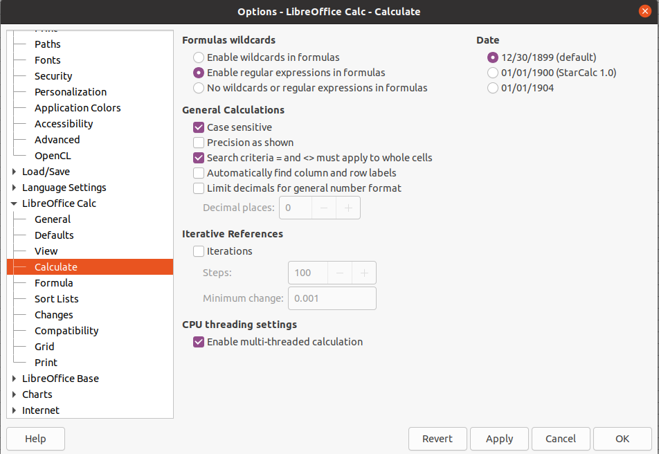
Using a Spreadsheet to Aggregate and Analyze the CSV Output

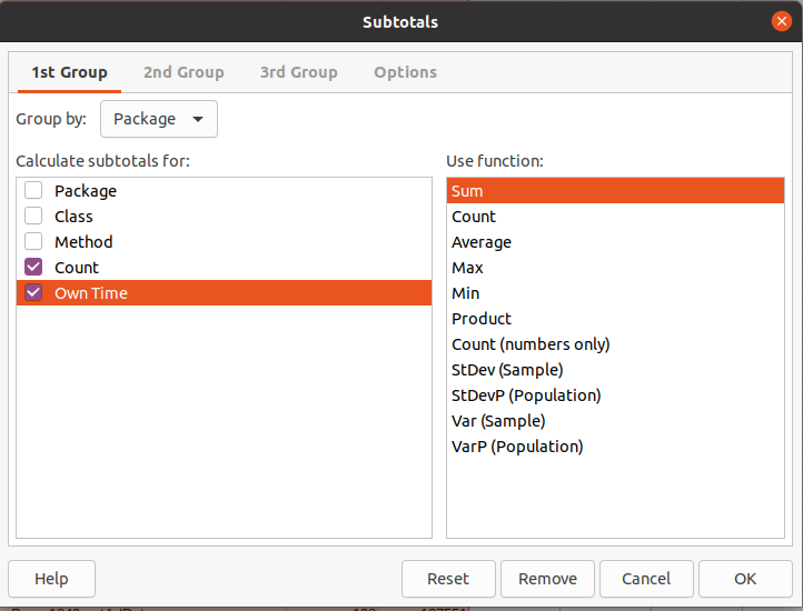
Using the HTML UI to Interpret Results¶

After executing ./server.sh -m0, beside the trace.csv file, a HTML UI is generated. Inside deploy/server/trace there are generated files which can be used to visualize the method tracing data:

index.html is the root file to be opened to visualize data. The Web page should be simple to use
- The left menu presents the root of the traced scenarios. Each such link opens a different scenario.
- The top menu presents the bucket traced.
- The table in the middle is the data from the selected scenario for the selected bucket.
data contains the server-side exported data regarding method tracing. Each folder inside is the root of a scenario. Each such folder has a JS per bucket which is included in the index.html file.
data/meta.js has information about overall statistics like: the name of the buckets, the name of the roots and the total elapsed time
js/loader.js is responsible for initializing the trace data for each scenario. This is the first JS which should be included in the index.html file.
js/trace.js is copied here as a resource and provides the basic functionality for the interface.
css/bootstrap.min.css is a bootstrap CSS used for interface styling.

Example of Using Method Tracing on Hotel GUI¶

Right now (Hotel_GUI rev. 252), the project is configured to allow -a and -m options. In order to retrieve some information on method tracing for the Hotel GUI project, one should run:

./deploy/server/server.sh -a to start the server with LTW
open a client using ./deploy/client/client.sh and go to place in application, which should be traced.
./deploy/server/server.sh -m1 to start tracing
do the scenario for which the tracing is intended
./deploy/server/server.sh -m0 to stop tracing
consult trace.csv

The trace_hotel_gui.csv results file is attached as an example. It was generated by tracing the login and some basic operations inside Hotel GUI.

Comparing Results¶

The most simple way of comparing results is by retrieving the CSV or HTML UI from two executions of the same scenario inside the target application.
These should be compared side-by-side as they usually generate the same scenarios/method tracing.

*TODO: think of a better way to display the performance delta between two H2 version. Maybe the HTML UI can be extended to load 2 data folders and compute delta.

Result-set Invalidation Tracing¶

AdaptiveQuery tracing is enabled/disabled together with Method Tracing.

The results are displayed in adaptive.csv and are split into two categories:

per query information
Each query displays data about it's state and methods called:
- The procedure where the AdaptiveQuery was defined (from the converted application).
- Number of tables joined.
- Scrolling status.
- Number of calls to a few important methods (invalidation, revalidation, etc.)
- Ratio between the invalidate and stateChanged methods.
- Ratio between the return type of the doubleCheckInvalidation method (true/false).
- A table containing predefined methods in which information about the total number of calls, calls before the first invalidation, calls between the first invalidation until the next revalidation, number of calls in preselect/dynamic mode, time executed in these two modes, percentage from the total number of calls of the methods called in these modes and total time executed by each method traced.
overview information
- Total number of queries.
- Total number of invalidated queries.
- Number of calls to a few important methods (invalidation, revalidation) and an average per query value for each one.
- Number of method calls made by all the queries.
- Number of scrolling/non-scrolling queries.
- A total table that sums the table defined for each query, but displays the average value obtained from all the queries for most of the values obtained from each query.
- A parent calls table with the purpose of displaying the number of AdaptiveQueries generated by a procedure.

The results of adaptive.csv file can be influenced by two final values declared in the AdaptiveQuery tracing class:

OUTPUT_ALL_QUERIES: Controls the displayed queries. When set to false, only queries that were invalidated are displayed. This flag provides easier access to important queries when tracing in a large application and is set to false by default.
PARENT_CALL_AMOUNT_LIMIT: Threshold representing the minimum amount of queries that a procedure call needs to generate in order to be displayed in the parent calls table. By default this value is set to 3.

Analyzing Large Heap Dumps¶

For large heap dumps, it may not be possible to load them with jhat or similar tools, for live OQL analysis, as the memory requirements may exceed the available RAM on the machine (for example, a binary file of 27GB was created when dumping 17GB of heap used by the FWD server, and this couldn't be loaded with jhat even if it was allowed to use 55GB of RAM).

It is possible to analyze these large heap dumps using Eclipse MAT, available here: https://www.eclipse.org/mat/downloads.php

Download and extract the Linux (x86_64/GTK+) version int ~/apps/mat. Edit the ~/apps/mat/MemoryAnalyzer.ini and add these parameters (adjust the Xmx and Xms accordingly to your system):

-vmargs
-Xms26144m
-Xmx48192m
-XX:+UseConcMarkSweepGC
-XX:+CMSParallelRemarkEnabled
-XX:+CMSClassUnloadingEnabled
-XX:+UseCMSInitiatingOccupancyOnly

Note that Eclipse MAT requires Java 11 or above to run. You will need to install a (non-default) JDK 11 and edit ~/apps/mat/ParseHeapDump.sh to add these lines, so MAT will use Java 11:

export JAVA_HOME=/usr/lib/jvm/java-11-openjdk-amd64/
export PATH=$JAVA_HOME/bin:$PATH
java --version

Once Eclipse MAT is installed and configured, follow these steps:

run the application scenario which is suspected of a memory leak, or other 'stress test' scenario. Wait for it to finish completely. Leave the FWD server running, if possible.
dump the FWD server heap:
```
jmap -dump:format=b,file=$PWD/heap_dump_PID.hprof PID
```
where PID is the process ID for the FWD server.

analyze this heap dump file with MAT:

cd ~/apps/mat
./ParseHeapDump.sh /path/to/heap_dump_PID.hprof org.eclipse.mat.api:suspects

where heap_file.hprof is the heap you want to analyze.

This will require disk space, so make sure you have free space at least the size of the heap file available, on the partition where the heap file is located. Once the analyze finishes, the report is in a zip file, in the same folder as the analyzed heap file. For the 'suspects' plugin, the report will show you some top-consumers, and you will have to confirm if these are real or not. For example, you can:

look where these instances are kept in FWD
attach a debugger to the FWD server
add breakpoints where these instances are created or added to collections
run the original scenario, wait for the breakpoint to hit and check if the collection where the instance is added contains a runaway number of instances
repeat as necessary

Other arguments for ParseHeapDump.sh are (from https://wiki.eclipse.org/MemoryAnalyzer/FAQ):

org.eclipse.mat.api:suspects argument creates a ZIP file containing the leak suspect report. This argument is optional.
org.eclipse.mat.api:overview argument creates a ZIP file containing the overview report. This argument is optional.
org.eclipse.mat.api:top_components argument creates a ZIP file containing the top components report. This argument is optional.

Once these reports are generated, you can open the heap dump in Eclipse MAT - create a script with a content like this, so Java 11 is used:

export JAVA_HOME=/usr/lib/jvm/java-11-openjdk-amd64/
export PATH=$JAVA_HOME/bin:$PATH

java --version

"$(dirname -- "$0")"/MemoryAnalyzer

And open the heap file.
----

Profiling through Persistence Loggers¶

One may use configurations specific to SQLStatementLogger or P2JQueryLogger in order to profile various SQLs or P2JQueries. These will be placed in the directory, under the persistence tag for global profiling, or under the database/<database-name> tag for database-specific profiling.

More information on what else can be logged can be found in PersistenceLogger.

SQLStatementLogger¶

An example of configuration for SQL profiling:

          <node class="container" name="sql-logging">
            <node class="string" name="enabled">
              <node-attribute name="value" value="TRUE"/>
            </node>
            <node class="boolean" name="profiling">
              <node-attribute name="value" value="TRUE"/>
            </node>
            <node class="double" name="min-time-threshold">
              <node-attribute name="value" value="0.5"/>
            </node>
            <node class="string" name="output-to-file">
              <node-attribute name="value" value="sql_%db.log"/>
            </node>
          </node>

In the above example, SQLs that are slower than 0.5 milliseconds will be logged in database-specific files (.log).

P2JQueryLogger¶

An example of configuration for P2JQuery profiling:

          <node class="container" name="p2j-query-logging">
            <node class="string" name="enabled">
              <node-attribute name="value" value="TRUE"/>
            </node>
            <node class="integer" name="processed-components">
              <node-attribute name="value" value="1"/>
            </node>
            <node class="boolean" name="profiling">
              <node-attribute name="value" value="TRUE"/>
            </node>
            <node class="double" name="min-time-threshold">
              <node-attribute name="value" value="0.01"/>
            </node>
            <node class="string" name="output-to-file">
              <node-attribute name="value" value="p2j-query_%db.log"/>
            </node>
          </node>

In the above example, P2J Queries that are slower than 0.01 milliseconds will be logged in database-specific files (.log).

VisualVMplugins.png (61.8 KB) Igor Skornyakov, 10/20/2021 09:24 AM

FWDMBeans.png (128 KB) Igor Skornyakov, 10/20/2021 09:32 AM

MBeansOps.png (127 KB) Igor Skornyakov, 10/20/2021 09:35 AM

hotel_trace.csv (268 KB) Alexandru Lungu, 10/21/2022 11:19 AM

subtotals_example.png (43 KB) Greg Shah, 10/28/2022 08:43 AM

libreoffice_regex_in_formula.png (95.8 KB) Constantin Asofiei, 10/28/2022 09:13 AM

Project

General

Profile

FWD

Wiki

Profiling¶

Introduction¶

How to Enable Tracing¶

Analysis Tips¶

Merged Callees¶

How to Find a Problematic Method¶

Bottlenecks in FWD¶

Bottlenecks in Converted Code¶

JMX MBean Instrumentation¶

Introduction¶

Design¶

Usage¶

Adding Tracepoints¶

JMX Instrumentation Types¶

TimeStat¶

Counter¶

MapCounter¶

QueryProfiler¶

LockTableUpdaterStat¶

Available Instrumentation Points¶

FWD Appserver Agent State Instrumentation¶

FWD Server - Persistence and ORM Instrumentation¶

FWD Server Runtime Instrumentation¶

FWD OpenClient Runtime Instrumentation¶

Other Miscellaneous Metrics¶

Persistence Subsystem Method Tracing¶

Setup¶

Enabling/Disabling at Runtime¶

Interpreting the CSV Results¶

Using the HTML UI to Interpret Results¶

Example of Using Method Tracing on Hotel GUI¶

Comparing Results¶

Result-set Invalidation Tracing¶

Analyzing Large Heap Dumps¶

Profiling through Persistence Loggers¶

SQLStatementLogger¶

P2JQueryLogger¶

`TimeStat`¶

`Counter`¶

`MapCounter`¶

`QueryProfiler`¶

`LockTableUpdaterStat`¶