Call Graph Visualization
Introduction
FWD Analytics provides a visual way to explore your code. This relies on the computed call graph, and allows you to dig into your application in a more friendly way. You will be able to view sub-graphs, filter using a specified file list (which can be the root list, a specified program or even a custom file list; this sub-graph will show all dependencies originating from or targeting the specified programs.
You will be able to customize the level of detail, zoom in and out, or navigate off-screen, away into other sub-graphs, using a specialized More node. Each graph component type will be identified by color and shape, with the links between the components labeled with the dependency type, which exists between these two components.
This chapter will describe how to identify the graph components, navigate through it and how to customize the visualization, to explore your code.
Tour of the Call Graph Visualization
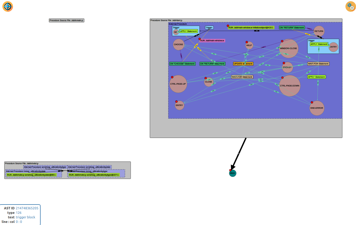
The Visualization screen is split into these parts:- Legend. There is a legend that can be accessed from the compass icon (in the top-left corner). To open it, click on the compass icon; to close it, click on the shown legend component.
- Settings. The visualization settings can be accessed from the gear box icon (in the top-right corner). This will be described in the Navigation section.
- Graph. The main visualization screen, with the graph components and dependencies (links) between them.
- AST Details. The currently highlighted AST component's details are shown in the bottom-left corner (only for AST components). For AST components (like
RUNstatements, function definitions, etc), you can useSHIFT-CLICKto highlight this code in the program's the source view screen.
All these parts can be seen here:
The legend will show you how to interpret each link and node, by their color. The legend is filtered, it only displays details for those node and link types that appear in the visible graph:

The graph visualization uses a grid layout to show the components; these will be ordered in such a way so the link overlapping is minimized and the top level components will not intersect. The top level components are container nodes (represented via rectangles), which can be:
- Procedure source code, which will have as sub-components the external procedure code, the internal procedures, user-defined functions and triggers; all these can be considered entry points into this program file.
- Class definitions, which will have as sub-components the class methods, constructors, destructors and property getters and setters; all these can be considered entry points into this program file.
- R-Code libraries, which will have as sub-components the defined internal procedures and user-defined functions which can be executed by other code.
- Native libraries, which will have as sub-components the native APIs called by your application.
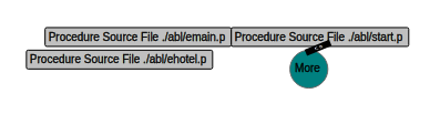
Each component which is enclosed in a procedure source file may contain one or more call-sites, as presented below:
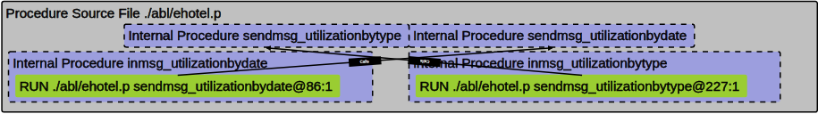
Here you can see the outer Procedure Source File rectangle for program start.p, which encloses the internal procedures, with their enclosed call-sites. A more complex program is presented below:
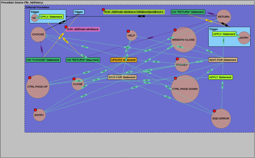
The container components, their enclosed call sites and all links will always be labeled. Beside the containers, the other shown components are:
- Non-container nodes, which may be call sites, external targets (like a missing resource, native process, etc) - these will always be a simple labeled rectangle.
- Events, represented by circles.
- The
Morecomponent, represented by a circle with theMoretext. This component can be used to navigate off-screen - the next section describes how to do this.
In all cases, you can hover the mouse over a graph node, and it will show you a tooltip with a more detailed description of that node.
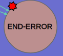
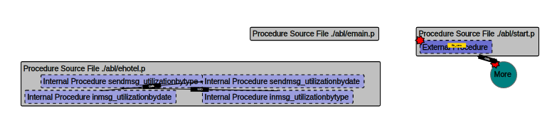
All components which have a star in the top-left corner allow you to show or hide the links which target components outside this source file; by default, links outside of the source file are hidden and the star is red; clicking it will show all these links and turn the star to green; clicking it again will turn it back to red, as all links are hidden. If the shown color is yellow, it means that some of the links are hidden, while some are visible. The following example shows an event which can execute a trigger outside the source file:
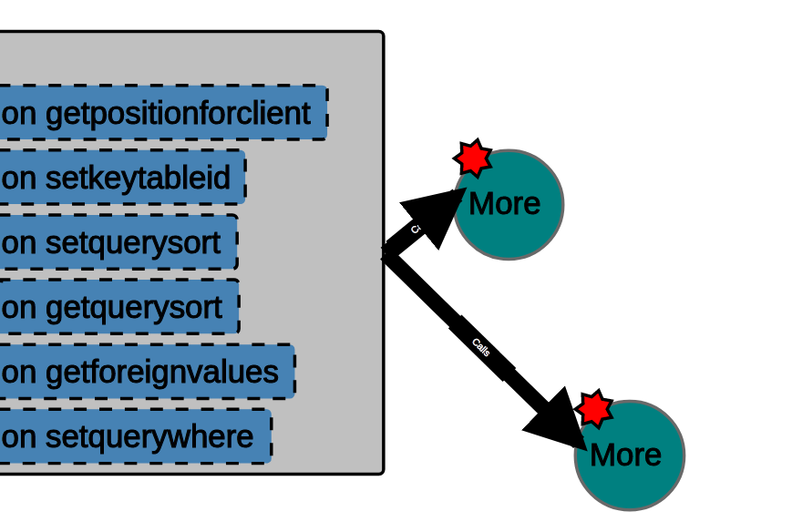
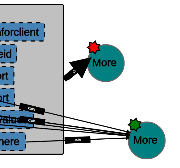
The links between the visualized components are weighted: when they are not expanded, a link will be thicker, depending on the number of inter-component dependencies (links). This can be easily seen if you expand a 'thick' link:
and after expanding the links for the lower More component:
Navigation
The settings window can be opened via the gearbox icon in the top-right corner:
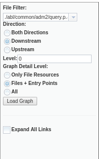
Each time you change a setting, press the Load Graph button to refresh the graph. If you don't want to apply the changes or to just close it, click on the blank background of the settings window.
Mouse Control
The visualized graph can be controlled via the mouse. This allows you to:
- Zoom. Zoom in or out, via the mouse scroll button/wheel. This will enhance or reduce the size of the graph, using a center point the current location of your mouse cursor. If you want to zoom in into a certain program, just place the mouse over that program and use the scroll upwards, to zoom in. Zoom out by using the mouse button/wheel to scroll downwards.
- Panning. Drag the graph sideways or vertically. Initially, you may notice that the graph is off screen: you can fix this by zooming out until a portion of the graph is visible, drag the graph to center it and zoom back in.
Each component is 'jailed' inside a pre-computed rectangular area; mouse allows you to click'n'drag the component, but it will not allow you to exit the 'jail'. In addition, the graph may ignore your change, as it tries to rebalance itself.
Applying Filters
By default, the graph visualization will start with the configured root list (see Defining the Root List for more details). The File Filter selection is populated by default with the Root List and Include All elements, plus all configured lists in the File List Filter section of FWD Analytics. This can be used to specify:
- Root List , which will include all programs defined as root entry points into your application.
- Include All, which will show the entire graph. WARNING - depending on the machine where the report server is executed and where the FWD Analytics browser page is opened, this may take a while to compute. It may be unusable, especially on a large project.
- Specify a custom list of programs by explicitly writing a comma-separated list of files, in the combo's text box. These file names must be AST file names, and project-relative; thus, for a program file named
./abl/foo/bar.p, the provided file name must be./abl/foo/bar.p.ast - Any other list of files as configured in the File List Filter section of FWD Analytics.
Changing Direction
The call graph is a directed graph; thus, you can customize the direction to follow when computing the dependencies for the vizualised graph. The possible settings are:
- Downstream - for a certain program, only its dependencies will be included. These are 'out edges' for a certain node, in the graph. This mode is the natural 'call graph' mode, where you can follow the links to determine which program(s) are reachable.
- Upstream - for a certain program, only the programs dependent on it will be included. These are 'in edges' for a certain node, in the graph.
- Both Direction - dependencies are followed in either way.
Graph Detail Level
The Expand All Links toggle box will show/hide the links which show dependencies between source files. By default, all links between source files are collapsed, and weighted - the more links that exist between two files, the thicker the link. Use the star in the top-left corner of a component, to show/hide those nodes which are adjacent to it.
The graph is built by doing a breadth-first traversal (BFS) of the graph, as deep as the number of specified levels; the visualized graph will all the reachable nodes, not exceeding the allowed number of levels. By default, when 0 levels are specified, only the filtered programs are shown, with More nodes used to identify dependencies to other programs. The deeper you go, the more complex your visualized graph will become.
Beside the graph depth level, it may be helpful to collapse some of the container nodes. By default, these containers are expanded and all their information (like internal procedures and their call sites) are displayed. If you find the visualized graph too complex, you can reduce this by specifying a detail level:
- Only File Resources will include only components which are files, like external programs, classes, schema files and external (or missing) resources.
- Files + Entry Points will include all File Resources (as described above), plus any 'entry point' into that file (these can be user-defined functions, triggers, class methods, etc).
- All will show everything.

Each image above shows the same visualized graph, with each available detail level.
Off-Screen Navigation
More nodes allow you to navigate to another program, which is one-level lower (than the shown files) in the graph traversal. Use the mouse left-click button and the SHIFT and CTRL keys, where:
- Pressing
CTRL-CLICKwill add the program represented by theMorenode to the filtered list. This allows you to keep your current graph and 'expand' all dependencies to/from the selected program. - Pressing
SHIFT-CLICKwill reduce the filtered list to the program represented by theMorenode. This allows you to view the sub-graph which has the selected program as its starting point.
Jump to Source View
If you SHIFT-CLICK (left mouse button while the SHIFT key is pressed) on any AST node, it will take you to the Source View associated with that AST node. This allows you to see node's source code and the AST in tree form.
Limitations and Known Issues
The visualized graph is intended to provide a way to walk into your source code. To avoid clutter, the graph will omit:
- The include sub-graph.
- Links from virtual functions (defined
IN SUPERorIN handle) or internal procedures (definedIN SUPER).
The graph layout sometimes may be unstable: it will always try to self-balance, but there are cases where it can get in an infinite loop, with two or more adjacent components switching place with each other. If this happens, try to 'catch' and drag a component with the mouse, to stop the animation.
When having a large number of source files on the visualized graph, the screen can get crowded (depending on your screen resolution); it may be worth it to limit the graph to show only the file resources, and once you reach a point of interest, show details for only that file resource.
The Include All filter, as it will show the complete graph, may get your browser in an unresponsive state. You can reduce the number of detail, use a file-resource detail, while following only the out links (Out Direction). In any case, this mode can be considered experimental, as for real life applications (with 1000s of programs), the screen most likely will become unusable.
When choosing the graph detail level, consider the visualized graph can grow exponentially: while level 1 may be usable, level 2 or more will bring too many nodes into the graph to be possible to follow it.
© 2004-2018 Golden Code Development Corporation. ALL RIGHTS RESERVED.